Algorithms
It’s a little tricky to define an algorithm, but informally we can use the term interchangeably with more well-known English words like recipe or procedure.
Definition: an algorithm is a finite sequence of unambiguous and effectively computable instructions that produce some intended result.
Let’s explore some of those terms in more detail:
- finite:
- An algorithm must terminate at some point. If it might go on forever, then we might never achieve the intended result.
- sequence:
- The instructions are ordered – first do this, then do that, etc. – and the order must be followed to achieve the correct result. (As an aside, there are parallel algorithms, in which the instructions are only partially ordered. We’ll ignore that distinction for now.)
- unambiguous:
- Each instruction must be specified precisely, so there can be no confusion as to what must be done. If multiple interpretations of the instruction are possible, it’s not an algorithm.
- computable:
- Each instruction must specify some task that can be performed. This gets a little theoretical, but there are some types of problems that no computer can solve in finite time. For now, let’s just take a simple example of an uncomputable instruction: “predict tonight’s lottery numbers.” Because the lottery is random, there’s no procedure we can follow to reliably predict it.
- result:
- We develop an algorithm to produce some specific answer. It could be a solution to a math problem, a stream of output, a modification of values stored in the memory, or whatever.

@hmason on Twitter
Notation
An algorithm is independent of the language or notation in which it is specified. The binary search algorithm can be written in Python or Java or Ruby, but they’re all the same algorithm.
One notation sometimes used for algorithms is called pseudo-code (where pseudo of course means “false” or “fake”). Unlike real code in a programming language, pseudo-code cannot be executed directly by a computer. However, because it’s based on English (with a little mathematical notation), it’s easier for untrained humans to understand.
Below is an example of an algorithm, written in pseudo-code, that will compute the factorial of a given integer, N. (The factorial is the result of multiplying all the numbers between 1 and N, so factorial of 4 is 1×2×3×4 = 24.)
Algorithm: factorial
- Let N be an integer > 0.
- Let K be 1.
- If N = 1 then output K and stop.
- Set K to K×N.
- Set N to N–1.
- Go back to step 3.
To understand this algorithm, we need to introduce the concept of a variable in programming. We use variables in mathematics too, but they’re a little different. In mathematics, a variable is a name given to a value, like x=5. In programming, a variable is a name given to a location in memory, which in turn can hold a value. The difference is that the value in the memory can be updated at a later time.
Let’s trace the algorithm. In step 1, we’re allowed to specify the value of N, as long as it is bigger than zero. This is a kind of input instruction. Let’s use 4, so that the algorithm computes the factorial of 4. In step 2, another variable K is named, but it’s initial value is 1. Here’s what that looks like:

Step 3 asks whether N=1. It does not, so we skip the rest of that instruction.
Step 4 updates a variable. We first compute the value of the expression: K×N = 1×4 = 4, and then we write that value to the box labeled K, replacing whatever was there before:

Step 5 updates the other variable. We first compute the value of the expression: N–1 = 4–1 = 3, and then we write that result to the box labeled N, replacing whatever was there before:

Step 6 says to go back to step 3. In step 3, N is still not 1, so we continue with the two updates again. This time, K×N = 4×3 = 12, and N–1 = 3–1 = 2:

N is still not 1, so we go through once more, producing these values for the two variables:

This time N=1, so in step 3 we output K and stop. By following this algorithm, we just computed the factorial of 4:
Output: 24By starting the same algorithm with a different value of N, we could have computed any factorial.
Another example
Here’s an algorithm you can try tracing yourself.
Algorithm:
- Let A,B be integers > 0.
- If A = B then output A and stop.
- If A < B then set B to B–A and go back to step 2.
- Otherwise set A to A–B and go back to step 2.
I won’t tell you what this algorithm produces, but try it starting with these values for A and B:
    A: 35
    B: 21
Then try these:
    A: 28
    B: 12
And finally these:
    A: 14
    B: 33
Do you see the pattern? What does the algorithm compute?
Sorting
One rich area of algorithms is sorting – putting things in some order, whether that’s alphabetical, numerical, chronological, or by size. There are many different sorting algorithms with different strengths and weaknesses. These videos introduce a few of them.
See also:
Speed
Whenever we talk about the “speed” of an algorithm, we have to consider the size of the input. In fact, we’re usually most concerned about how the size of the input impacts the running time, as that size increases. Maybe for sorting 8 elements, there isn’t much difference. But when we increase that to 50 or 1,000, dramatic differences may emerge.
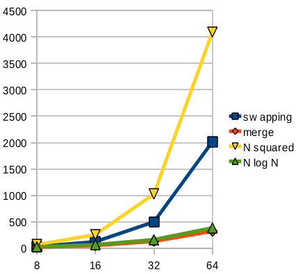
Below is a graph comparing the number of comparisons for selection vs. merge sort, and also showing the lines N² and N·log₂(N), which are characterizations of these different approaches. You can see that the selection sort is somewhat less than N², however, they do grow large in the same awful way.