Perceptrons

Basics

To begin exploring this area, we started with the simplest artificial neural networks, known as perceptrons. This formulation began with McCulloch and Pitts in 1943.

We have a graph in which both nodes (circles) and edges (lines) are assigned real numbers in some range, typically 0..1 or -1..+1, but other ranges can be used too. Numbers assigned to nodes are called activation levels, and numbers assigned to edges are called weights.

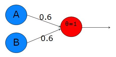
Sample Perceptron from this overview

In this perceptron, let’s call the two input nodes (left layer) A and B, and the output node is C. The upper edge weight will be \(w_a\) and the lower edge weight is \(w_b\). The main calculation is just a weighted average: \(C = A·w_a + B·w_b\).

But then we also apply a function to the result, to adjust its range and kind of “snap” it into a positive or negative result (activated or inactive). This function can be a simple “step” with a given threshold \(t\), such as \(t=0.5\) or \(t=1.0\):

\[ f(x) = \biggl\{\begin{array}{ll} 0 & \mbox{if}\; x < t\\ 1 & \mbox{if}\; x \ge t\\ \end{array} \]

Step function, with threshold \(t=0\). [Source]

Later on, we may use a more sophisticated function that smooths out the discontinuity at the threshold, like this one, called the Sigmoid function:

\[ f(x) = \frac{1}{1+e^{-x}} \]

The “logistic” sigmoid (formula above), centered on \(x=0\). [Wikimedia]

It’s interesting to see if we can make perceptrons emulate the Boolean logic operators, like AND, OR, NOT, XOR. The perceptron above, with weights \(w_a=0.6\) and \(w_b=0.6\) implements OR:

A B  C = f(A*Wa + B*Wb)
0 0  f(0*0.6 + 0*0.6) = f(0)   = 0
0 1  f(0*0.6 + 1*0.6) = f(0.6) = 1  (because 0.6 > t)
1 0  f(1*0.6 + 0*0.6) = f(0.6) = 1
1 1  f(1*0.6 + 1*0.6) = f(1.2) = 1

Here we’re using the step function with threshold \(t=0.5\).

We can implement Boolean AND with \(w_a=0.4\) and \(w_b=0.4\):

A B  C = f(A*Wa + B*Wb)
0 0  f(0*0.4 + 0*0.4) = f(0)   = 0
0 1  f(0*0.4 + 1*0.4) = f(0.4) = 0  (because 0.4 < t)
1 0  f(1*0.4 + 0*0.4) = f(0.4) = 0
1 1  f(1*0.4 + 1*0.4) = f(0.8) = 1  (because 0.8 > t)

XOR

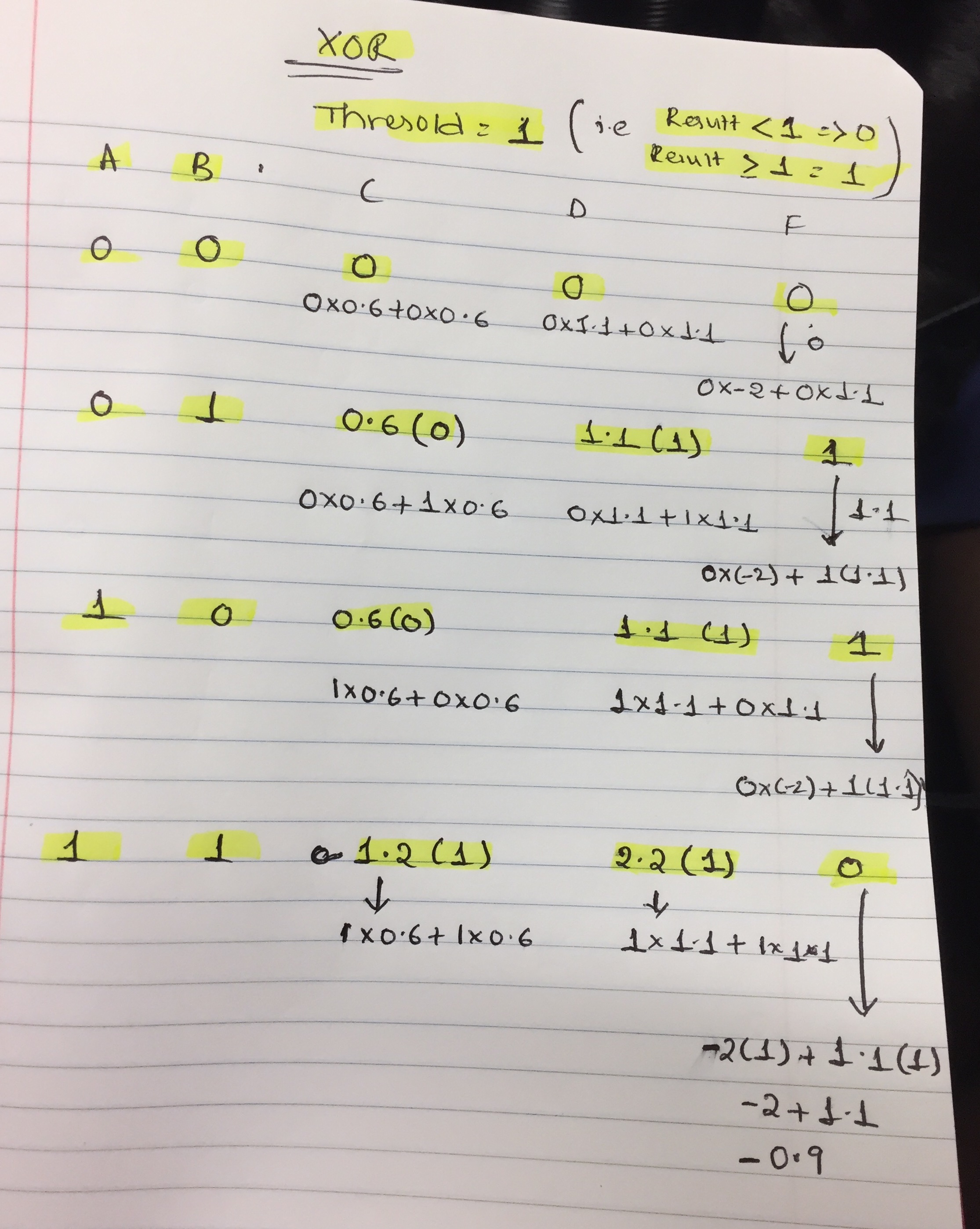
A problem arises with the XOR function. Minsky and Papert showed that this simple perceptron model cannot encode XOR. (And their influence set back research into artificial neural networks for a decade or more!) A perceptron can model (and learn) any function that is linearly separable, but XOR is not.

The trick to making this model more powerful is to add a “hidden” layer between the input nodes and the output node. Then you fully-connect the nodes of the input layer with those in the hidden layer. That produces a graph with five nodes and six edges:

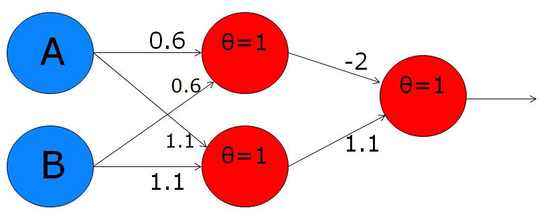
XOR implementation with hidden layer

The threshold value for the step function is indicated by θ (theta). The work below is by one of my graduate students, Priya.

Full resolution

Implementation

At first I tried to simulate the delta rule in a spreadsheet – this worked for learning AND, OR. When I tried to learn NAND using a bias input, I wasn’t getting it to work. Can you?

Here is the start of a Python implementation:

# Perceptrons!

class TwoStepFun(object):
    """A step function with configurable threshold.

    >>> 3+3
    6
    >>> f1 = TwoStepFun()
    >>> f1.threshold
    0.5
    >>> f1(0.4)
    0
    >>> f1(0.6)
    1

    >>> f2 = TwoStepFun(1)
    >>> f2(0.99)
    0
    >>> f2(-1.2)
    0
    >>> f2(1.001)
    1
    """
    def __init__(self, threshold=0.5):
        self.threshold = threshold

    def __call__(self, value):
        if value < self.threshold:
            return 0
        else:
            return 1

class Perceptron(object):
    """Represent a perceptron with 2 inputs, bias.

    >>> p1 = Perceptron(TwoStepFun(1))
    >>> p1.weights = [0.6, 0.6, 0.0]
    >>> bits = [0,1]
    >>> [p1(a,b) for a in bits for b in bits]
    [0, 0, 0, 1]

    >>> p2 = Perceptron(TwoStepFun(0.5))
    >>> p2.weights = [0.6, 0.6, 0.0]
    >>> bits = [0,1]
    >>> [p2(a,b) for a in bits for b in bits]
    [0, 1, 1, 1]
    """
    def __init__(self, transfer):
        from random import random
        self.transfer = transfer
        self.weights = [random()*4-2,
                        random()*4-2,
                        random()*4-2]

    def __call__(self, x0, x1):
        avg = (x0 * self.weights[0] +
               x1 * self.weights[1] +
               1  * self.weights[2])
        return self.transfer(avg)

    def learn(self, x0, x1, target):
        pass #TODO

if __name__ == "__main__":
    import doctest
    doctest.testmod()