Sorting
Swapping pairs
We first looked at this algorithm where you go through all pairs in an organized fashion, and swap them if they are out of order relative to each other.
    Bee  Eel  Ant  Dog  Cat
     1    2    3    4    5

The pairs are:
     1,2  1,3  1,4  1,5  = 4
          2,3  2,4  2,5  = 3
               3,4  3,5  = 2
                    4,5  = 1
Total comparisons:
     4 + 3 + 2 + 1 = 10
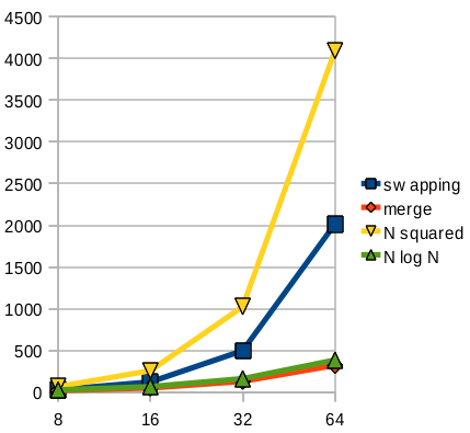
The general formula for the number of comparisons needed for N words is , which is roughly N². As the size of your data set increases, the number of comparisons grows very fast:
   N     N(N-1)/2
 -----   --------
   5       10
   8       28
  16      120
  32      496
  64     2016
Merge sort
Next, we looked at merge sort, using playing cards. The idea is to divide and conquer: split 8 cards into 2 groups of 4, then 4 groups of 2. Once you have just a pair, sorting is easy: just compare them. Then you have to merge all the groups together. Here’s a demo similar to mine, but with cups instead of playing cards.
Our computations in class of the number of comparisons for merge sort were these – they’re way smaller than for the swapping sort above.
   N     comparisons
 -----   --------
   8     17
  16     49
  32     129
  64     321
Speed
Whenever we talk about the “speed” of an algorithm, we have to consider the size of the input. In fact, we’re usually most concerned about how the size of the input impacts the running time, as that size increases. Maybe for sorting 8 elements, there isn’t much difference. But when we increase that to 50 or 1,000, dramatic differences may emerge.
Below is a graph comparing the number of comparisons for swapping vs. merge sort, and also showing the lines N² and N·log₂(N), which are characterizations of these different approaches. You can see that the swapping sort is somewhat less than N², however, they do grow large in the same awful way.
