Assignment 1 solutions
Sun Sep 16
These declarations make this file into an executable module that runs embedded test cases.
{-# LANGUAGE TemplateHaskell #-}
import HApprox ((@?~))
import Test.Tasty.HUnit (testCase, (@?=))
import Test.Tasty.TH (defaultMainGenerator)
main = $(defaultMainGenerator)
Warm-up: volume of a sphere
For this question, we will see how to submit and receive feedback on Haskell function definitions with the Mimir platform. Below is what we call “starter code.” It consists of a module declaration and the beginning of a function definition called volumeSphere.
Try this: following the equals sign, type a floating-point number, such as 9.2. Don’t change anything else in the starter code. Then hit the “Run tests” button. You should see that most (probably all) of the tests have failed.
Click on one of the test names, where it says “Debugging information available.” You will see some feedback that includes a chunk like this:
expected: 4.1887902047863905
 but got: 9.2
That one pertains to the example volumeSphere 1. The test expects the result to be 4.1887902047863905 but instead the result was 9.2.
Dismiss the debugging information, and now change the expression in the program to 4.1887902047863905. When you press “Run tests” again, this time it should pass the first test but fail the others.
Now, replace your floating-point constant with the actual expression which will define this function correctly. You can find it in the course notes for 5 September. With that definition in place, the code should compile and all the tests should pass. Once the tests pass, you can move on to the next question.
Solution
Tests
case_volumeSphere_1 = volumeSphere 1 @?~ 4.1887902047863905
case_volumeSphere_3p5 = volumeSphere (3 + 5) @?~ 2144.660584850632
case_volumeSphere_3_p5 = volumeSphere 3 + 5 @?~ 118.09733552923254
Quadratic equation
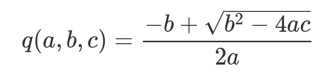
Define this mathematical function using Haskell. Again, do not change the starter code, just add your expression after the equals sign. The square-root function in Haskell is spelled sqrt.
Solution
Tests
case_quadratic_2_9_3   = quadratic 2 9 3       @?~ -0.36254139118231254
case_quadratic_1_n1_n1 = quadratic 1 (-1) (-1) @?~  1.618033988749895
case_quadratic_2_8_6   = quadratic 2 8 6       @?~ -1.0
case_quadratic_1_30_pi = quadratic 1 30 pi     @?~ -0.1050878704703262
Temperature conversion
For this problem, you should write two functions, called celsiusToFahrenheit and fahrenheitToCelsius. They should perform conversions between the two temperature scales. (You can look up the formulas on the web.) This time the starter code has the module declaration (leave that alone), but you must write the function declarations yourself.
Solution
Tests
case_0C_in_F     = celsiusToFahrenheit   0   @?~  32
case_100C_in_F   = celsiusToFahrenheit 100   @?~ 212
case_212F_in_C   = fahrenheitToCelsius 212   @?~ 100
case_32F_in_C    = fahrenheitToCelsius  32   @?~   0
case_body_temp_F = fahrenheitToCelsius  98.6 @?~  37
case_body_temp_C = celsiusToFahrenheit  37   @?~  98.6
case_C_F_roundtrip = do
let rt c = fahrenheitToCelsius (celsiusToFahrenheit c) @?~ c
rt 18.2
rt pi
rt 39872
rt (-37.119)case_F_C_roundtrip = do
let rt f = celsiusToFahrenheit (fahrenheitToCelsius f) @?~ f
rt 18.2
rt pi
rt 39872
rt (-37.119)Cartesian distance metrics
There are several different ways to calculate a distance between two points on a Cartesian plane. Below is a demonstration. Points are specified as pairs of numbers \((X,Y)\). The two points shown here are \((1,2)\) and \((5,4)\). Think of the first as a starting point of a journey (green) and the second as the end point (red).
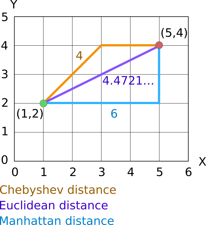
The most straightforward calculation may be Manhattan distance. It’s just the sum of the distances in both dimensions, like walking along city blocks — go 4 blocks East then 2 blocks North, the total distance is then 6 blocks. You just have to be cautious about calculating those distances, because they should never be negative. In this example, the X distance comes from \(5 - 1 = 4\), but if you’re given the points in the reverse order you might calculate \(1 - 5 = -4\). So we use the absolute value, usually notated with bars on each side of the expression: \(| 1 - 5 | = 4\). In Haskell, however, the absolute value is provided by the function abs.
The Euclidean distance takes a square root of the sum of squared distances in each dimension. Its formula is derived directly from the Pythagorean theorem, you can find it online if you need to.
The Chebyshev distance is a more flexible alternative to Manhattan distance. It counts diagonal moves as being the same distance as horizontal/vertical moves. Think of the movements of a queen on a chess board. Its calculation is simply the maximum of the distances in each dimension. You can get the maximum of two values in haskell with, for example, max 5 2.
Name your functions just manhattan, euclidean, and chebyshev. They should each take two pairs as arguments.
Solution
Tests
case_chebyshev_horiz    = chebyshev (3,2) (9,2) @?~ 6
case_chebyshev_negative = chebyshev (-3,-4) (-8,9) @?~ 13
case_chebyshev_unit_sq  = chebyshev (0,0) (1,1) @?~ 1
case_chebyshev_vertical = chebyshev (3,2) (3,6.3) @?~ 4.3
case_euclid_horiz = euclidean (3,2) (9,2) @?~ 6
case_euclid_negative = euclidean (-3,-4) (-8,9) @?~ 13.92838827718412
case_euclid_unit_sq = euclidean (0,0) (1,1) @?~ sqrt 2
case_euclid_vertical = euclidean (3,2) (3,5.7) @?~ 3.7case_manhattan_horiz = manhattan (3,2) (9,2) @?~ 6
case_manhattan_negative = manhattan (-3,-4) (-8,9) @?~ 18
case_manhattan_unit_sq = manhattan (0,0) (1,1) @?~ 2
case_manhattan_vertical = manhattan (3,6.1) (3,2) @?~ 4.1Fast exponentiation
The starter code includes a recursive function, powerSlow, to calculate exponents with a non-negative integer power. For example, powerSlow 2 5 produces 32. (Trace it yourself to see how it works!)
Your task is to create a function powerFast. It looks almost exactly the same as powerSlow, but includes one extra clause (before the otherwise) that will take a shortcut when the exponent is an even number. The shortcut works through an application of this formula:
\[ x^{2y} = (x^y)^2 \]
So the \(2y\) on the left side of the formula indicates that the exponent is an even number (a multiple of two). You can then take the power using half that exponent, and square the result. This results in substantially fewer multiplications when the exponent is large.
You should define your own square function to use in powerFast; one test case requires this.
Solution
powerFast x n
  | n < 0 = error "Negative exponent"
  | n == 0 = 1
  | even n = square (powerFast x (div n 2))
  | otherwise = x * powerFast x (n-1)
Tests
case_powerFast_3_0  = powerFast 3 0  @?= 1
case_powerFast_4_15 = powerFast 4 15 @?= 1073741824
case_powerFast_5_16 = powerFast 5 16 @?= 152587890625
case_square_71      = square 71      @?= 5041
Primes
A prime number is an integer that has exactly two factors: one, and itself. The number 1, however, is not considered to be prime. So the first few prime numbers are 2, 3, 5, 7, 11, 13.
Define a helper function using the symbolic operator notation slash-question-mark: (/?). This can be used as an infix operator to determine whether a number is divisible by another number (with no remainder). It returns a Boolean. For example:
ghci> 3 /? 2
False
ghci> 18 /? 3
True
ghci> 18 /? 4
False
Next, you can define isPrime n. It can check whether any number in the range [2..n-1] divides n. (It also must ensure that n > 1.)
Finally, a twin prime is a pair of neighboring odd numbers that are both primes. For example 11 and 13 are both prime so they are referred to as twins. Define a function isFirstTwinPrime n that determines whether n is the first of a pair of twin primes.
Solution
Tests
case_8_div_by_3 = 8 /? 3     @?= False
case_8_div_by_4 = 8 /? 4     @?= True
case_isPrime_1  = isPrime  1 @?= False
case_isPrime_2  = isPrime  2 @?= True
case_isPrime_19 = isPrime 19 @?= True
case_isPrime_21 = isPrime 21 @?= False
case_count_primes_to_1000 =
  length (filter isPrime [1..1000]) @?= 168
case_first_10_twin_primes =
  take 10 (filter isFirstTwinPrime [1..]) @?=
  [3,5,11,17,29,41,59,71,101,107]