Interpreters and trees
10 February 2016
Interpreters
Compilers and interpreters, of course, have a lot to do with programming languages. We have at least three roles for languages:
The source language is the language that the compiler or interpreter takes as input.
The target language is the language the compiler outputs. (Interpreters don’t have a target language.)
The host language is the language the compiler or interpreter is written in.
Things get interesting when the source language and host language are the same. For example, a C compiler that is written in C or a Java virtual machine (a low-level interpreter) written in Java. Such systems raise the question “what compiles the compiler?” This leads to a process called bootstrapping, which is fraught with complexity – we may discuss it in more depth later.
Identifying these three roles also allows us to easily distinguish between a compiler and an interpreter. With a compiler, once we have produced the target code it can execute with no more involvement from the host language. In contrast, with an interpreter the host language’s runtime system is active and directly involved in executing the source program.
One decision point in creating an interpreter is the level of processing at which we begin interpreting. It’s rare to interpret directly from the character string representing the source program. Instead, we might run the lexical analyzer and interpret a sequence of tokens – that’s called a syntax-directed interpreter (pattern 24, chapter 9 in the book). Or we might do a full parse in advance and then interpret from the parse tree or abstract syntax tree (pattern 25).
The advantage of doing lexical analysis and (possibly) parsing before interpreting is especially evident in code with loops. When we iterate through the same piece of code many times, it would be wasteful to re-discover the same sequence of tokens (or the same tree structure) each time through.
Writing Pico programs
Related to assignments 2 and 3, it’s helpful to understand a little better how PicoScript works by writing programs in it. In class, I proposed writing a PicoScript program to calculate Collatz sequences. Starting with any integer \(n>0\), we produce the next integer as follows. If \(n\) is even, divide it by two. If \(n\) is odd, then calculate \(3n+1\). The numbers in the sequence can oscillate wildly up and down, but with every starting integer ever tried the sequence leads to the number \(1\). However, there is still no formal proof that the sequence terminates for every integer.
In PicoScript we have a mod operator that can be used to distinguish even or odd:
7 2 mod % [1]8 2 mod % [0]and then we can apply 0 eq to turn those into Booleans:
7 2 mod 0 eq % [false]8 2 mod 0 eq % [true]Now we have the ifelse operator that can take a Boolean and two blocks of code. It uses the Boolean to decide which block to execute. So in one block, we divide by two (integer division with idiv) and in the other we use 3 mul 1 add to calculate \(3n+1\).
7 2 mod 0 eq {2 idiv} {3 mul 1 add} ifelse % Error: stack underflowThe problem that happened here is that the original integer, 7, gets consumed as soon as you calculate its modulus.
So we need to dup the number before we apply the 2 mod so that a copy of it is still around when we want to divide or multiply:
7 dup 2 mod 0 eq {2 idiv} {3 mul 1 add} ifelse % [22]Here’s the same code, but starting with an even number:
10 dup 2 mod 0 eq {2 idiv} {3 mul 1 add} ifelse % [5]So this is the core logic of any Collatz program. We can use it either to generate the whole sequence from some starting point, or to count how long it takes to reach the end. Either way, let’s define it as a new operator:
/collatzRule {
    dup 2 mod 0 eq
    {2 idiv}
    {3 mul 1 add}
  ifelse
} def
Here are some more examples of applying it:
31 collatzRule % [94]161 collatzRule % [484]122 collatzRule % [61]32 collatzRule % [16]Now we want to loop it somehow, to generate the sequence. PicoScript has a few loop operators, but the while is a convenient one in this case. If the number is greater than one, we keep going. Again, we need to use dup at the beginning of each block to prevent it from consuming our only copy of the current number.
/collatzSeq {
  {dup 1 gt}
  {dup collatzRule}
  while
} def
17 collatzSeq % [17, 52, 26, 13, 40, 20, 10, 5, 16, 8, 4, 2, 1]27 collatzSeq % [27, 82, 41, 124, 62, 31, 94, 47, 142, 71, 214,
% 107, 322, 161, 484, 242, 121, 364, 182, 9, 274,
% 137, 412, 206, 103, 310, 155, 466, 233, 700,
% 350, 175, 526, 263, 790, 395, 1186, 593, 1780,
% 890, 445, 1336, 668, 334, 167, 502, 251, 754,
% 377, 1132, 566, 283, 850, 425, 1276, 638, 319,
% 958, 479, 1438, 719, 2158, 1079, 3238, 1619,
% 4858, 2429, 7288, 3644, 1822, 911, 2734, 1367,
% 4102, 2051, 6154, 3077, 9232, 4616, 2308, 1154,
% 577, 1732, 866, 433, 1300, 650, 325, 976, 488,
% 244, 122, 61, 184, 92, 46, 23, 70, 35, 106, 53,
% 160, 80, 40, 20, 10, 5, 16, 8, 4, 2, 1]Now suppose that instead of generating the whole sequence, we only need to know its length. To achieve that we’ll use a similar while loop but keep the current Collatz number on the top of the stack, and the number of steps we’ve taken just below that.
/collatzLength {
    0 exch              % Initialize number of steps taken
    { dup 1 gt }        % Have we reached 1 yet?
    { collatzRule       % Generate next number (but don't keep current one)
      exch 1 add exch   % Increment number of steps taken
    }
    while               % Loop the above procedures
    pop                 % Pop the final 1, leaving only the count
} def
32 collatzLength % [5]27 collatzLength % [111]63728127 collatzLength % [949]Tree representations
Much of the work of a compiler is analyzing and rewriting trees. So the data structures and implementation patterns we use for trees are very important. There are two general kinds of trees that represent the source program:
A parse tree is a literal indication of what rules from the grammar can be invoked to produce the program text. The trees shown in the notes on parsing and grammars were all parse trees.
An abstract syntax tree (AST) is a simplification of the parse tree. It eliminates nodes that are no longer needed – generated by rules that existed only to encode operator precedence, for example. It also emphasizes the operations that are expected to happen rather than artifacts from the grammar.
For a good example of the difference between a parse tree and an AST, consider arithmetic expressions that contain parentheses, such as x*(y+3). The only role of those parentheses is to override the usual order of operations. They ensure that the addition in parentheses happens before the multiplication. But once we have this expression in tree form, the parentheses are redundant. Therefore the AST will eliminate them.
In a parse tree, the leaves are terminals (tokens) and the interior nodes are non-terminals. So the actual operations being performed: + and * sit at the leaves. The AST turns that around so the operation is at the root and the operands are its children. Compare the two figures below.
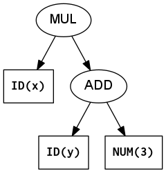
Abstract Syntax Tree for x*(y+3)
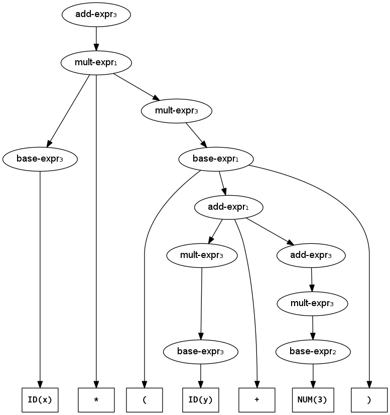
Parse tree for x*(y+3) (using the precedence-segregated expression grammar)
Homogeneous AST
The simplest way to represent an AST is to use a single node class which stores a list of child nodes. Each node also keeps track of its type (what syntactic unit it represents) and usually a few other fields needed for some of the node types. This is called a homogeneous (same kind) representation. For example, here is a Node class to represent ASTs for the calculator language.
class Node {
    enum Type {
        PROG,     // Children are a sequence of statements
        ASSIGN,   // Child 0 is expr, ID stored too
        PRINT,    // Child 0 is expr
        ADD,      // The binary ops: child 0 is left, child 1 is right
        SUB,
        MUL,
        DIV,
        NUM,      // Numeric constant, no children
        ID        // Identifier, no children
    }
    Type type;          // What type of node is this?
    Node[] children;    // Uniform place to store child nodes
    BigInteger integer; // Used for NUM only
    String id;          // Used for ASSIGN and ID
}
You can see the complete class in the absyn folder of the cs664pub repository. In addition to the above fields, we add to the Node class some constructors to create nodes of different types. Here is the most generic possible constructor – you just provide the type and a list of children. (The three dots are Java notation for variadic arguments.)
    public Node(Type type, Node... children) {
        this.type = type;
        this.children = children;
    }
That constructor will work just fine for creating AST nodes representing binary operators (two children) and whole programs (arbitrary number of children).
    Node expr = new Node(Node.Type.ADD, expr1, expr2);
    Node prog = new Node(Node.Type.PROG, stm1, stm2, stm3, stm4, stm5);
For some other node types, it’s very useful to have custom constructors. Here’s one that initializes a number using a Java integer (converting it to BigInteger in the process):
    public Node(int x) {
        this.type = Type.NUM;
        this.integer = BigInteger.valueOf(x);
    }
And then two other custom constructors for variables and assignment:
    public Node(String id) {
        this.type = Type.ID;
        this.id = id;
    }

    public Node (String id, Node expr) {
        this.type = Type.ASSIGN;
        this.id = id;
        this.children = new Node[] {expr}; // Create array with one node
    }
Now that we finished with the constructors, it’s also useful to override the toString method so it shows something sensible. I like to use Lisp notation, where each interior node of the tree is wrapped in parentheses. The node type appears first inside the left parenthesis, and then the other children follow, separated by white-space. For example, the AST for the infix source language expression x*(y+3) would appear in prefix Lisp notation as (MUL x (ADD y 3)). Here is the toString definition for Node:
    @Override
    public String toString() {
        // Handle NUM and ID first -- those are the leaf types.
        if(type == Type.NUM) {
            return integer.toString();
        }
        else if(type == Type.ID) {
            return id;
        }
        else {
            // Now we've got an interior node, so wrap in parentheses
            StringBuilder buf = new StringBuilder("(");
            buf.append(type);
            if(type == Type.ASSIGN) {     // For assignment, insert ID
                buf.append(' ');          // before the expr node.
                buf.append(id);
            }
            for(Node child : children) {  // For each child,
                buf.append(' ');
                buf.append(child);        // Invoke toString on child
            }
            buf.append(")");
            return buf.toString();
        }
    }
Finally, we can bring all that together in a main program that constructs trees, prints, and executes them.
public class HomogeneousAST {
    public static void main(String[] args) {
        // The following builds a tree representing the program:
        // x=391; y=(x+1)/2; print y*y
        Node exprA =
                new Node(Node.Type.DIV,
                        new Node(Node.Type.ADD,
                                new Node("x"),
                                new Node(1)),
                        new Node(2));
        Node y = new Node("y");
        Node exprB = new Node(Node.Type.MUL, y, y);
        Node prog =
                new Node(Node.Type.PROG,
                        new Node("x", new Node(391)),
                        new Node("y", exprA),
                        new Node(Node.Type.PRINT, exprB));
        // Print and then interpret the program
        System.out.println(prog);
        interpret(prog);
    }
    // etc.
}
See the full definition, with the interpret method in the absyn/src folder of cs664pub. Running the main program produces:
(PROG (ASSIGN x 391) (ASSIGN y (DIV (ADD x 1) 2)) (PRINT (MUL y y)))
38416
Heterogeneous AST
Another way to represent an AST is to use different classes for AST nodes that have different requirements. They often form a class hierarchy, as shown in the inheritance diagram. This approach means we can more accurately reflect the expectations of the language: the distinction between statements and expressions, for example – represented here as abstract classes.
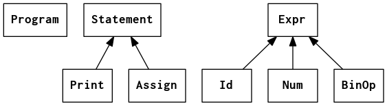
Class inheritance diagram for heterogeneous AST for calculator language
There can still be some sharing when different nodes have similar requirements – thus we have a BinOp class rather than a separate class for each operator: Add, Sub, Mul, etc. Below is a sample of the class declarations for an assignment statement – see HeterogeneousAST.java for the rest.
abstract class Statement {
    abstract void execute(HashMap<String, BigInteger> memory);
}

class Assign extends Statement {
    String id;
    Expr e;

    public Assign(String id, Expr e) {
        this.id = id;
        this.e = e;
    }

    @Override
    public String toString() {
        return "(ASSIGN " + id + " " + e + ")";
    }

    @Override
    void execute(HashMap<String, BigInteger> memory) {
        memory.put(id, e.evaluate(memory));
    }
}
The main program using the Heterogeneous AST looks similar to the previous one, except now we refer explicitly to different classes like Num, Id, Assign, and Print rather than everything being a Node.
public class HeterogeneousAST {
    public static void main(String[] args) {
        // The following builds a tree representing the program:
        // x=391; y=(x+1)/2; print y*y
        Expr exprA =
                new BinOp(BinOp.Op.DIV,
                        new BinOp(BinOp.Op.ADD,
                                new Id("x"),
                                new Num(1)),
                        new Num(2));
        Expr y = new Id("y");
        Expr exprB = new BinOp(BinOp.Op.MUL, y, y);
        Program prog = new Program(
                new Assign("x", new Num(391)),
                new Assign("y", exprA),
                new Print(exprB)
        );
        System.out.println(prog);
        prog.interpret();
    }
}
Also, when analyzing or rewriting trees using a heterogeneous representation, it’s a little easier to refer to fields with meaningful names rather than always using an array of nodes.
The output of this program using the heterogeneous AST is exactly the same as before:
(PROG (ASSIGN x 391) (ASSIGN y (DIV (ADD x 1) 2)) (PRINT (MUL y y)))
38416